In order to compare abiotic variables such as wind and wave action along the South African coastline, large historical datasets for temperature, wave and wind were analysed and accessed.

Wave and wind data

Wind and wave action were important variables in this study as they were hypothesised to exhibit a direct influence on coastal water temperatures; consequently, they were investigated for their impact on seawater temperature at specific sites along the South African coastline. Wind and wave data were obtained from the South African Weather Service (SAWS), and were provided at three-hour resolutions. Specific wind and wave characteristics were measured, namely, wave height (hs), wave period (tp), wave direction (dir), wind direction (dirw) and wind speed (spw). The data were then used to model short–crested waves, generated by the wind into the coastal environment, using the wave model Simulating Waves in the Nearshore (SWAN). SWAN enables the extraction of wave parameters from specific gridded locations in the nearshore. A resolution of 200m was modelled at both 7 and 15m isobaths.

## ── Attaching packages ───────────────────────────────────────────────────────────────────────────────────── tidyverse 1.3.0 ──

## ✔ ggplot2 3.2.1     ✔ purrr   0.3.3
## ✔ tibble  2.1.3     ✔ dplyr   0.8.3
## ✔ tidyr   1.1.1     ✔ stringr 1.4.0
## ✔ readr   1.3.1     ✔ forcats 0.4.0

## ── Conflicts ──────────────────────────────────────────────────────────────────────────────────────── tidyverse_conflicts() ──
## ✖ dplyr::filter() masks stats::filter()
## ✖ dplyr::lag()    masks stats::lag()

## Loading required package: magrittr

## 
## Attaching package: 'magrittr'

## The following object is masked from 'package:purrr':
## 
##     set_names

## The following object is masked from 'package:tidyr':
## 
##     extract

## 
## Attaching package: 'zoo'

## The following objects are masked from 'package:base':
## 
##     as.Date, as.Date.numeric

## 
## Attaching package: 'lubridate'

## The following object is masked from 'package:base':
## 
##     date

## 
## Attaching package: 'circular'

## The following objects are masked from 'package:stats':
## 
##     sd, var

## Loading required package: RColorBrewer

Loading in the wind and wave data. It is important to remember that the data used in this script was created in the previous scripts.

load("data/wave_data.RData")
load("data/SACTN_daily_clusters_sub.RData")

Converting the 3-hour resolution wave data into daily data. https://cran.r-project.org/web/packages/circular/circular.pdf (Pg 130). The circular function creates circular objects around the wind and wave direction. The wave and wind direction was collected every three hours and by using the circular function we calcuated the daily mean wave and wind direction. There is a numerically large gap between 360 and 2 where as in degrees its not as large. The circular mean function returns the mean direction of a vector of circular data.

wave_daily <- wave_data %>%
  mutate(date = as.Date(date)) %>%
  group_by(site, num, depth, date) %>%
  summarise(dir_circ = mean.circular(circular(dir, units = "degrees")),
            dirw_circ = mean.circular(circular(dirw, units = "degrees")),
            spw_circ = mean.circular(circular(spw, units = "degrees")),
            hs_circ = mean.circular(circular(hs, units = "degrees")),
            tp_circ = mean.circular(circular(tp, units = "degrees")))
# save(wave_daily, file = "data/wave_daily.RData")

Here I are splitting the daily wave data into depths of 7m and 15m respectivley

sites_complete_7a <- wave_daily %>%
  filter(depth == "7m")

sites_complete_15a <- wave_daily %>%
  filter(depth == "15m")

Now i match the SACTN seawater temperature data with the wave data

SACTN_daily_clusters_sub_1 <- SACTN_daily_clusters_sub %>% 
  separate(index, into = c("site", "src"), sep = "/", remove = FALSE)

try1 <- function(df) {
  func1 <- df %>% 
    left_join(sites_complete_7a, by = c("site", "date")) %>% 
    na.trim() %>% 
    group_by(site)
    return(func1)
}
try2 <- function(df) {
  func2 <- df %>% 
    left_join(sites_complete_15a, by = c("site", "date")) %>% 
    na.trim() %>% 
    group_by(site)
    return(func2)
}

SACTN_daily_clusters_7a <- try1(df = SACTN_daily_clusters_sub_1)
SACTN_daily_clusters_15a <- try2(df = SACTN_daily_clusters_sub_1)

Temperature and wave comparison

temp_wave_compare <- function(df){
  df1 <- df %>% 
    dplyr::mutate(year = year(date), 
                  week = week(date)) %>% 
    dplyr::select(-date) %>% 
    tidyr::gather(key = variable, value = value, 
                  -c(index:src, year, week, length:depth)) %>% 
    na.omit() %>% 
    ungroup() %>% 
    group_by(index, year, week, variable) %>% 
    na.omit() %>% 
    dplyr::summarise(value = mean(value, na.rm = T)) %>% 
    arrange(index, year, week) %>% 
    group_by(index, variable) %>% 
    mutate(index2 = 1:n())
  ggplot(data = df1, aes(x = index2)) +
    geom_line(aes(y = value, colour = variable, group = )) +
    facet_grid(variable~index, scales = "free_y")
}

temp_wave_compare(SACTN_daily_clusters_7a)

temp_wave_compare(SACTN_daily_clusters_15a)

Temperature and wave comparison

temp_wave_compare <- function(df){
  df1 <- df %>% 
    dplyr::mutate(year = year(date), 
                  week = week(date)) %>% 
    dplyr::select(-date) %>% 
    tidyr::gather(key = variable, value = value, 
                  -c(index:src, year, week, length:depth)) %>% 
    na.omit() %>% 
    ungroup() %>% 
    group_by(index, year, week, variable) %>% 
    na.omit() %>% 
    dplyr::summarise(value = mean(value, na.rm = T)) %>% 
    arrange(index, year, week) %>% 
    group_by(index, variable) %>% 
    mutate(index2 = 1:n())
  ggplot(data = df1, aes(x = index2)) +
    geom_line(aes(y = value, colour = variable, group = )) +
    facet_grid(variable~index, scales = "free_y")
}

temp_wave_compare(SACTN_daily_clusters_7a)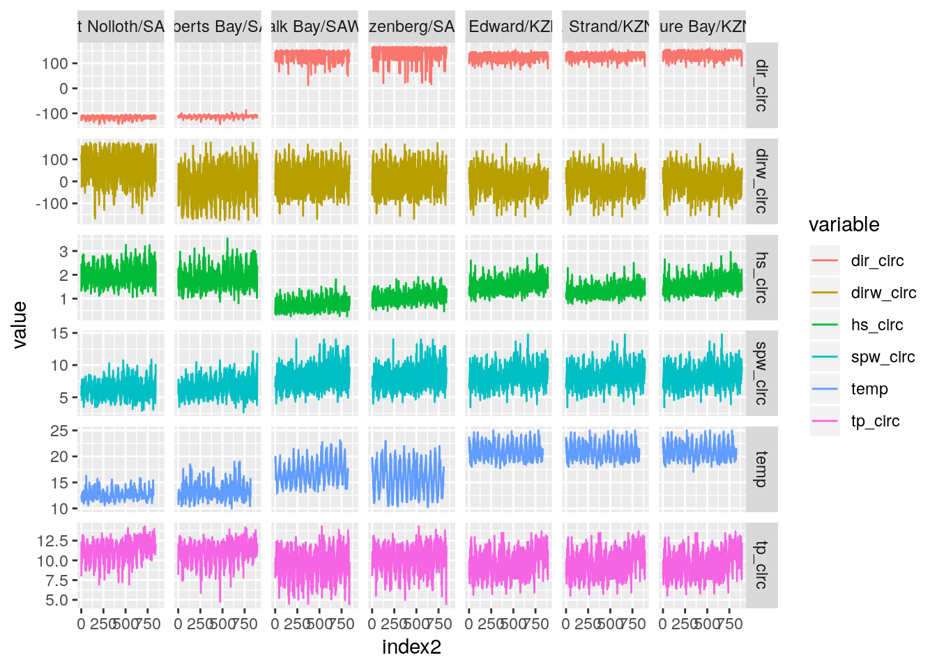

temp_wave_compare(SACTN_daily_clusters_15a)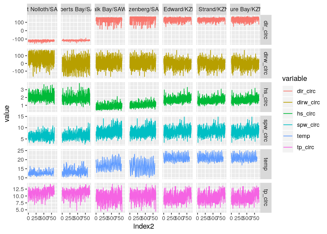

Calculating the R2 value of each of the variables

temp_wave_R2_ <- function(df){
  results <- df %>% 
    select(-index, -src, -date, -length, -c(num:depth)) %>%
    gather(key = variable, 
           value = value,
           -cluster, -site, -temp) %>%
    group_by(cluster, site, variable) %>%
    na.omit() %>% 
    nest() %>%
    mutate(model = purrr::map(data, ~lm(temp ~ value, data = .))) %>%
    unnest(model %>% purrr::map(glance)) %>%
    select(cluster:variable, adj.r.squared, p.value) %>% 
    arrange(cluster, site) %>% 
    mutate(adj.r.squared = round(adj.r.squared, 2),
           p.value = round(p.value, 4)) %>% 
        dplyr::rename("R^2" = adj.r.squared) %>% 
    dplyr::rename(P = p.value) %>% 
    dplyr::rename(Cluster = cluster) %>% 
    dplyr::rename(Site = site) %>% 
    dplyr::rename(Variable = variable) 
  return(results)
  }

#SACTN_7_R2 <- SACTN_daily_clusters_7a %>% 
 #temp_wave_R2_()
#SACTN_15_R2 <- SACTN_daily_clusters_15a %>% 
 # temp_wave_R2_()

Some visualisation

wave_daily_renamed <- wave_daily %>% 
  dplyr::rename(spd = spw_circ) %>%
  dplyr::rename(dir = dirw_circ) 

p.wr2 <- plot.windrose(data = wave_daily_renamed,
              spd = "spd",
              dir = "dir")

R> Hadley broke my code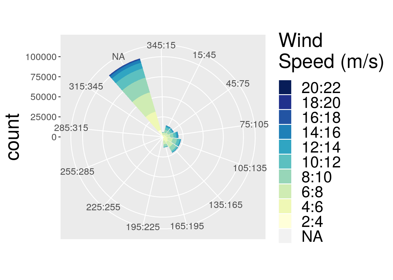

p.wr3 <- p.wr2 + facet_wrap(.~ site, ncol = 4, nrow = 5) +
  theme(strip.text.x = element_text(size = 25))
p.wr3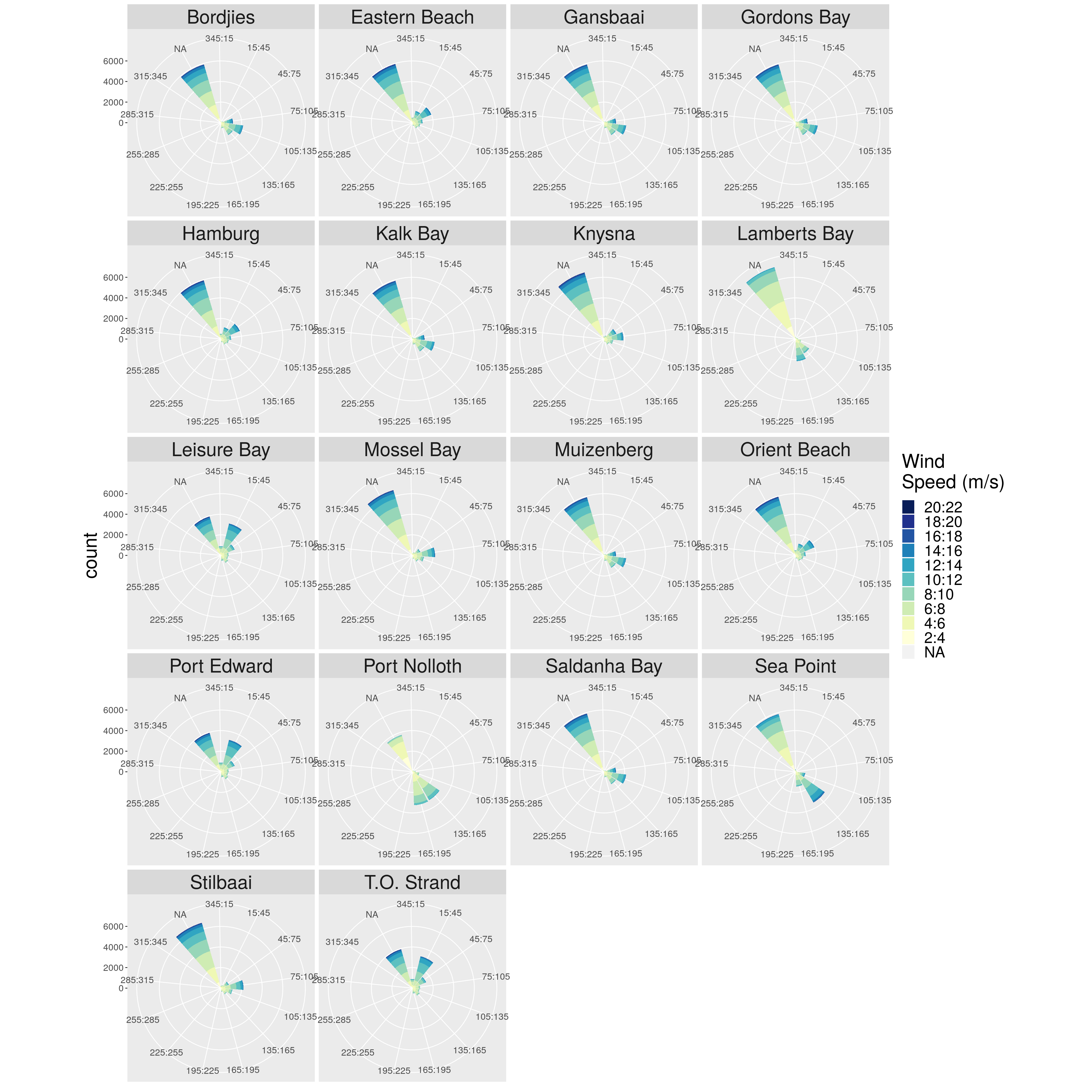

Figure 1: Windrose diagram representing the wind direction and speed for each of the sites

wave_daily_renamed <- wave_daily %>% 
  dplyr::rename(spd = hs_circ) %>%
  dplyr::rename(dir = dir_circ) 

p.wr2 <- plot.waverose(data = wave_daily_renamed,
              spd = "spd",
              dir = "dir") 

R> Hadley broke my code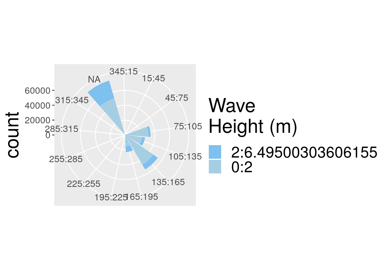

p.wave <- p.wr2 + facet_wrap(~site,
                            ncol = 4, nrow = 5) +
    theme(strip.text.x = element_text(size = 25))
p.wave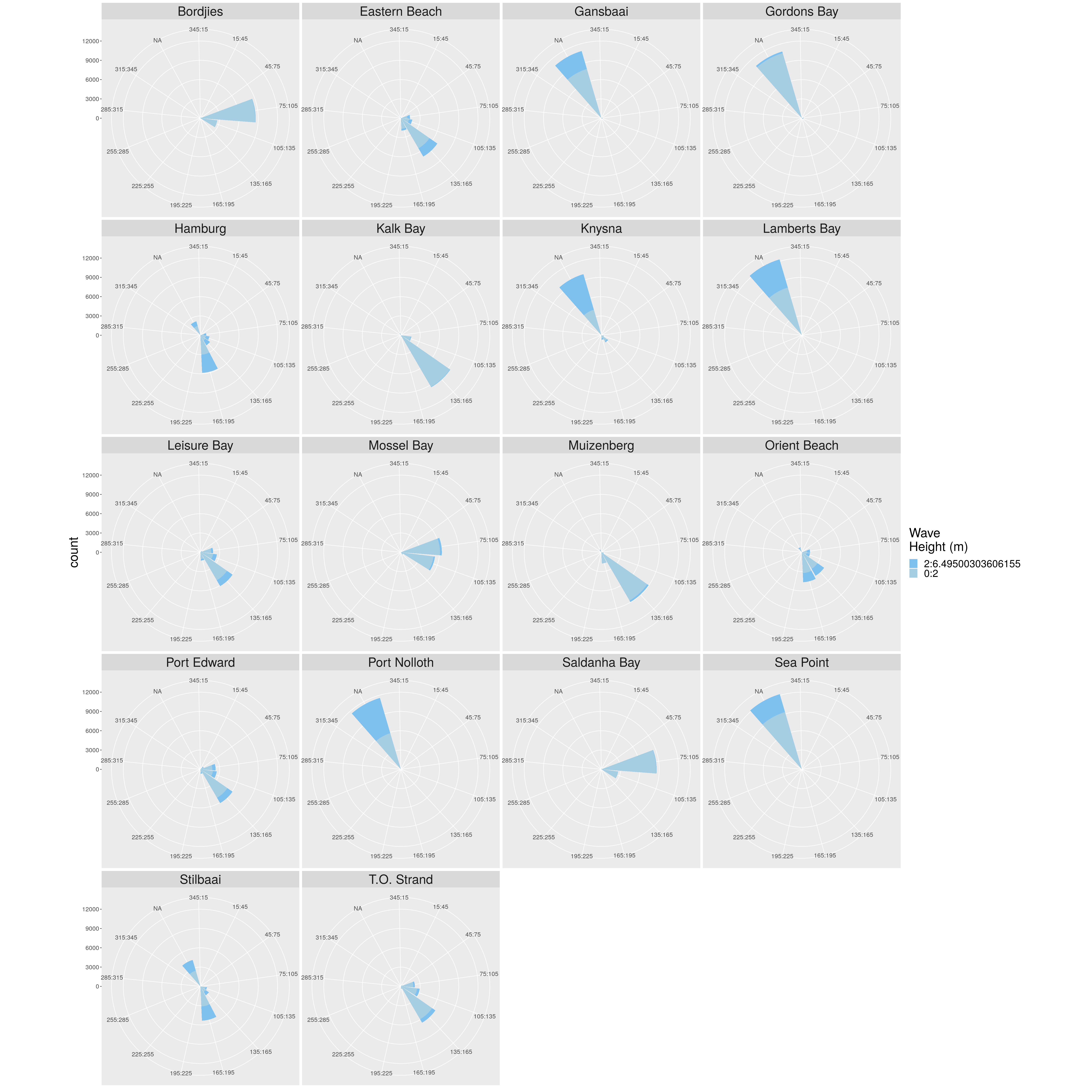

Figure 2: Windrose diagram representing the wind direction and speed for each of the sites