Global plot of SST
Mapping Eastern boundry upwelling
Coastal upwelling is a major oceanographic process driven by prominent currents near Eastern Boundary Upwelling Systems (EBUS) (Bakun and Nelson, 1991; Messié et al., 2009; Gruber et al., 2011; Pegliasco et al., 2015, Brady et al., 2019). EBUS include the California (CCS), Humboldt (HCS), Canary (CnCS) and Benguela (BCS) current systems (Figure 1), with each of these significantly impacting their associated coastal systems. These systems are characterised as vast regions of coastal ocean occurring along the western shores of continents bordering the Pacific and Atlantic Oceans (Bakun, 1990; Pauly and Christensen, 1995; Bakun et al., 2015, Bakun et al., 2010). EBUS span a wide range of latitudes and are therefore spatially heterogeneous environments. The CCS experiences significant natural variability from sources such as El Niño-Southern Oscillation (ENSO) and the Pacific Decadal Oscillation with important ecosystem consequences. The CnCS is heavily influenced by the North Atlantic Oscillation. The HCS environmental and biological diversity are also heavily influenced by ENSO. The BCS is unique as it experiences interannual variability in the physical and biological conditions relate to the Benguela Niños and Pacific ENSO. In the south, the BCS is largely influenced by the variability in the Agulhas current (García-Reyes, et al., 2015).
# 1: Setup environment ----------------------------------------------------------------------------------------------------
library(tidyverse) # Base suite of functions
## ── Attaching packages ───────────────────────────────────────────────────────────────────────────────────── tidyverse 1.3.0 ──## ✔ ggplot2 3.2.1 ✔ purrr 0.3.3
## ✔ tibble 2.1.3 ✔ dplyr 0.8.3
## ✔ tidyr 1.1.1 ✔ stringr 1.4.0
## ✔ readr 1.3.1 ✔ forcats 0.4.0## ── Conflicts ──────────────────────────────────────────────────────────────────────────────────────── tidyverse_conflicts() ──
## ✖ dplyr::filter() masks stats::filter()
## ✖ dplyr::lag() masks stats::lag()library(raster)## Loading required package: sp##
## Attaching package: 'raster'## The following object is masked from 'package:dplyr':
##
## select## The following object is masked from 'package:tidyr':
##
## extractlibrary(sf)## Linking to GEOS 3.7.2, GDAL 2.4.2, PROJ 5.2.0library(ggspatial)
library(rnaturalearth)
library(rnaturalearthdata)
library(PBSmapping)##
## -----------------------------------------------------------
## PBS Mapping 2.72.1 -- Copyright (C) 2003-2021 Fisheries and Oceans Canada
##
## PBS Mapping comes with ABSOLUTELY NO WARRANTY;
## for details see the file COPYING.
## This is free software, and you are welcome to redistribute
## it under certain conditions, as outlined in the above file.
##
## A complete user guide 'PBSmapping-UG.pdf' is located at
## /home/amieroh/R/x86_64-pc-linux-gnu-library/3.6/PBSmapping/doc/PBSmapping-UG.pdf
##
## Packaged on 2019-03-14
## Pacific Biological Station, Nanaimo
##
## All available PBS packages can be found at
## https://github.com/pbs-software
##
## To see demos, type '.PBSfigs()'.
## -----------------------------------------------------------library(viridis)## Loading required package: viridisLitelibrary(plotdap)## Registered S3 method overwritten by 'hoardr':
## method from
## print.cache_info httrlibrary(heatwaveR) # For detecting MHWs
# cat(paste0("heatwaveR version = ", packageDescription("heatwaveR")$Version))
library(FNN) # For fastest nearest neighbour searches
library(tidync) # For a more tidy approach to managing NetCDF data
# library(SDMTools) # For finding points within polygons
library(lubridate)##
## Attaching package: 'lubridate'## The following object is masked from 'package:base':
##
## dateload("data/OISST_global.RData") # Downloaded one year of global OISST data
load("data/site_squares.RData") # Making the squares showing the EBUS regions
OISST_global <- OISST_global %>%
mutate(lon = ifelse(lon > 180, lon - 360, lon))
map_base <- ggplot2::fortify(maps::map(fill = TRUE, col = "grey80", plot = FALSE)) %>%
dplyr::rename(lon = long) %>%
mutate(group = ifelse(lon > 180, group+9999, group),
lon = ifelse(lon > 180, lon-360, lon))
ggplot() +
geom_raster(data = OISST_global, aes(x = lon, y = lat, fill = temp), show.legend = TRUE) +
geom_polygon(data = map_base, aes(x = lon, y = lat, group = group)) +
geom_rect(data = site_squares, aes(xmin = xmin, xmax = xmax, ymin = ymin, ymax = ymax),
colour = "red", fill = NA, size = 0.75) +
annotate("text", label = "D", x = 4.0, y = -25.0,
size =5, angle = 0, colour = "black") +
annotate("text", label = "C", x = -25.0, y = 29.5,
size =5, angle = 0, colour = "black") +
annotate("text", label = "B", x = -88, y = -30,
size =5, angle = 0, colour = "black") +
annotate("text", label = "A", x = -133, y = 40.0,
size =5, angle = 0, colour = "black") +
scale_x_continuous(breaks = seq(-150, 150, by = 50),
labels = c("150°W", "100°W", "50°W", "0", "50°E", "100°E", "150°E")) +
scale_y_continuous(breaks = seq(-60, 60, by = 30),
labels = c("60°S", "30°S", "0", "30°N", "60°N")) +
coord_quickmap(ylim = c(-78.5, 90), expand = FALSE) +
scale_fill_gradientn("SST (°C)", values = scales::rescale(c(-1, 7,19,26)),
colors = c("lightcyan1", "orchid1", "skyblue", "blue3")) +
labs(x = NULL, y = NULL) +
theme_set(theme_grey()) +
theme_grey() +
theme(panel.border = element_rect(fill = NA, colour = "black", size = 1),
axis.text = element_text(colour = "black", size = 20, family = "Palatino"),
axis.title = element_text(colour = "black", size = 20, family = "Palatino"),
axis.ticks = element_line(colour = "black"),
axis.ticks.length = unit(0.4, "cm"),
legend.text=element_text(size=15, family = "Palatino"),
legend.title = element_text(size = 15, family = "Palatino"))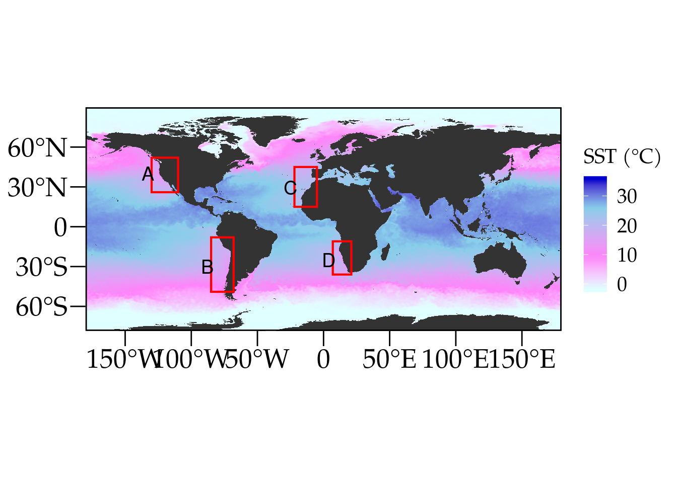
Amieroh Abrahams
Scientist with a passion for data, statistics; the ocean and the oceangraphic processes associated with it.