2 - Clustering and plotting

May 23, 2020 10 min read R

Welcome back! I hope that the first blog was useful for its scientific insight and adding to your coding and plotting skills.

The intention of this blogs is to show the approach and R scripts used to analyse the possible reasons for temperature variation between sites within the same cluster along the coast of South Africa and the controlling influences of temperatures within coastal zones.

Startup

First we need to find, install and load various packages. These packages will be available on CRAN and can be accessed and installed in the usual way.

knitr::opts_chunk$set(
  comment = "R>",
  warning = FALSE,
  message = FALSE
)

library(tidyverse)
## ── Attaching packages ───────────────────────────────────────────────────────────────────────────────────── tidyverse 1.3.0 ──
## ✔ ggplot2 3.2.1     ✔ purrr   0.3.3
## ✔ tibble  2.1.3     ✔ dplyr   0.8.3
## ✔ tidyr   1.1.1     ✔ stringr 1.4.0
## ✔ readr   1.3.1     ✔ forcats 0.4.0
## ── Conflicts ──────────────────────────────────────────────────────────────────────────────────────── tidyverse_conflicts() ──
## ✖ dplyr::filter() masks stats::filter()
## ✖ dplyr::lag()    masks stats::lag()
library(ggpubr)
## Loading required package: magrittr
## 
## Attaching package: 'magrittr'
## The following object is masked from 'package:purrr':
## 
##     set_names
## The following object is masked from 'package:tidyr':
## 
##     extract
library(zoo)
## 
## Attaching package: 'zoo'
## The following objects are masked from 'package:base':
## 
##     as.Date, as.Date.numeric
library(lubridate)
## 
## Attaching package: 'lubridate'
## The following object is masked from 'package:base':
## 
##     date
library(ggrepel)
library(FNN)
library(stringr)
library(viridis)
## Loading required package: viridisLite
library(gridExtra)
## 
## Attaching package: 'gridExtra'
## The following object is masked from 'package:dplyr':
## 
##     combine
library(dplyr)
source("functions/scale.bar.func.R")
## 
## Attaching package: 'maps'
## The following object is masked from 'package:purrr':
## 
##     map
## Loading required package: sp
## Checking rgeos availability: TRUE
source("functions/earthdist.R") # lies in the folder labeled funtions

It is now necessary to load the daily SACTN temperature dataset. The SACTN dataset was the primary source of temperature data used in this study. This dataset consisted of coastal seawater temperatures for 129 sites along the coast of South Africa, measured daily from 1972 until 2017. Of these, 80 were measured using hand-held thermometers and the remaining 45 were measured using UTRs. The duration and extent of the recordings per sitewere uneven, with the longest time series in the dataset being that of Gordons Bay, recorded by the South African Weather Service (SAWS). Data collected for this region started on 13 September 1972 and concluded on 26 January 2017, with recordings still continuing daily. During the 1970s, a total of 11 time series began recording. A further 53 entries were added during the 1980s, 34 entries were added during the 1990s, and 18 entries were added during the 2000s. Recordings are still ongoing at many of these sites.

load("data/SACTN_daily_v4.2.RData")
load("data/site_list_v4.2.RData")
load("data/sa_provinces.RData")
load("data/south_africa_coast.RData")
load("data/sa_coast.Rdata")

Clustering the sites using the k-means results in the previous blog: Creating a cluster index whilst only selecting cluster 6 Working with at least one decade of data for each of the sites along the coast, and excluding time series with temperature data collected deeper than a five metres.

set.seed(10)
site_list$cluster <- as.factor(kmeans(site_list[,c(15, 18:19)], 6)$cluster)

site_list_clusters <- site_list %>% 
  filter(length >= 3650, depth <= 5)

SACTN_daily_clusters <- SACTN_daily_v4.2 %>% 
  left_join(site_list[,c(4, 13, 21)], by = "index") %>% 
  filter(index %in% site_list_clusters$index)

Site selection

With the sites now split into six clusters, the next step is to reduce the number of sites per cluster down to a manageable, but still representative, sub-sample of the whole. This is done primarily for two reasons. The first, simply, is to allow for the comparisons to be more readily interpretable by humans. The second more objective reason is to allow for an equal amount of sampling per cluster. The East coast is much more heavily sampled than the rest and so this imbalance must be addressed. The criteria that must be considered for the sub-samples are that both instrument types (UTR and thermometer) are present, and as many sources are included as are possible. The statistical characteristics of the seawater temperature dataset was used as to guide analyses into the suitability of the time series which allows us to produce an accurate assessment of temperature variation between sites located within the same cluster. The precision, length and decadal trend of the time series for each of the sites were adjusted systematically.

# First simply divide up the site list by cluster
sites_1 <- site_list_clusters %>%
  filter(cluster == 1)
sites_2 <- site_list_clusters %>%
  filter(cluster == 2)
sites_3 <- site_list_clusters %>%
  filter(cluster == 3)
sites_4 <- site_list_clusters %>%
  filter(cluster == 4)
sites_5 <- site_list_clusters %>%
  filter(cluster == 5)
sites_6 <- site_list_clusters %>%
  filter(cluster == 6)

# I then grouped the sub-samples by source and took the longest time series
# When fewer than 4 sources were present, I took the next longest time series etc.
sites_1_sub <- sites_1 %>%
  group_by(src) %>%
  filter(length %in% head(length, 2)) %>%
  ungroup()

sites_2_sub <- sites_2 %>%
  group_by(src) %>%
  filter(length %in% head(length, 4)) %>% 
  ungroup() %>% 
  slice(c(1,2,3))

sites_3_sub <- sites_3 %>%
  group_by(src) %>%
  filter(length %in% head(length, 4)) %>% 
  ungroup() %>% 
  slice(c(1,2,5))

sites_4_sub <- sites_4 %>% 
  group_by(src) %>%
  filter(length %in% head(length, 2)) %>%
  ungroup() %>% 
  slice(c(2,3,4))

sites_5_sub <- sites_5 %>% 
  group_by(src) %>%
  ungroup() %>% 
  slice(c(1,4,10))

sites_6_sub <- sites_6 %>% 
  group_by(src) %>%
  filter(length %in% head(length, 4)) %>% 
  ungroup() %>% 
  slice(c(1,2,3))

# This then creates subsets of the four sites per cluster
# Though we may want to consider the distance between sites as well...
# Anyway, for now I stitch them together to be used as a further index
# for subsetting the daily data

site_list_sub <- rbind(sites_1_sub, sites_2_sub, sites_3_sub, sites_4_sub, sites_5_sub, sites_6_sub)
SACTN_daily_clusters_sub <- SACTN_daily_clusters %>%
  filter(index %in% site_list_sub$index)
#save(site_list_sub, file = "data/site_list_sub.RData")

Mapping the site locations

Map showing the location of each site within each of the six clusters

site_coordinates1 <- filter(site_list_sub, cluster == 1) %>% 
  select(site, lon, lat)

site_coordinates2 <- filter(site_list_sub, cluster == 2) %>% 
  select(site, lon, lat)

site_coordinates3 <- filter(site_list_sub, cluster == 3) %>% 
   select(site, lon, lat)

site_coordinates4 <- filter(site_list_sub, cluster == 4) %>% 
  select(site, lon, lat)

site_coordinates5 <- filter(site_list_sub, cluster == 5) %>% 
  select(site, lon, lat)

site_coordinates6 <- filter(site_list_sub, cluster == 6) %>% 
  select(site, lon, lat)

mapping_plot <- function(df, xy = "salmon"){
  mapping <- df %>% 
    ggplot(aes(x = lon, y = lat)) +
    geom_polygon(data = south_africa_coast, aes(group = group), fill = "white") +
    coord_cartesian(xlim = c(12, 36), ylim = c(-32, -20)) +
    geom_path(data = sa_provinces, aes(group = group)) +
    geom_point(data = df, colour = xy, size = 4)  +
    # geom_label_repel(data =df, aes(x = lon, y = lat, label = site), 
    #                  size = 0.5, box.padding = 2, nudge_x = -0.5, nudge_y = 0.2, 
    #                  segment.alpha = 0.4, force = 0.1) +
    coord_equal(xlim = c(15, 35), ylim = c(-37, -27)) +
    annotate("text", label = "INDIAN\nOCEAN", x = 35.00, y = -34.0, size = 3.0, angle = 0, colour = "black") +
    annotate("text", label = "ATLANTIC\nOCEAN", x = 16.00, y = -37.0, size = 3.0, angle = 0, colour = "black") +
    annotate("text", label = "Agulhas", x = 31.7, y = -31.7, size = 3, angle = 53, colour = "black") +
    scale_x_continuous(labels = scales::unit_format(unit = "°E", sep = "")) +
    scale_y_continuous(labels = scales::unit_format(unit = "°S", sep = "")) +
    labs(x = NULL, y = NULL) +
    coord_cartesian(xlim = c(10.5, 39.5), ylim = c(-39.5, -25.5), expand = F) +
    # scaleBar(lon = 32.0, lat = -38.7, distanceLon = 200, distanceLat = 50, 
    #          distanceLegend = 90, dist.unit = "km", arrow.length = 100,
    #          arrow.distance = 130, arrow.North.size = 3) +  
    coord_equal() +
    theme(aspect.ratio = 1)  +
    theme_bw() +
    theme(panel.border = element_rect(fill = NA, colour = "black", size = 1),
          axis.text = element_text(colour = "black", size = 6),
          axis.title = element_text(colour = "black", size = 6))
  return(mapping)
}

map_clus1 <- mapping_plot(df = site_coordinates1, xy = "salmon")
map_clus2 <- mapping_plot(df = site_coordinates2, xy = "darkgoldenrod4")
map_clus3 <- mapping_plot(df = site_coordinates3, xy = "springgreen4")
map_clus4 <- mapping_plot(df = site_coordinates4, xy= "lightskyblue")
map_clus5 <- mapping_plot(df = site_coordinates5, xy= "steelblue3") 
map_clus6 <- mapping_plot(df = site_coordinates6, xy= "mediumorchid1") 

final_map_combined_A <- ggarrange(map_clus1, map_clus2, map_clus3, map_clus4, map_clus5, map_clus6, ncol = 2, nrow = 3)
final_map_combined_A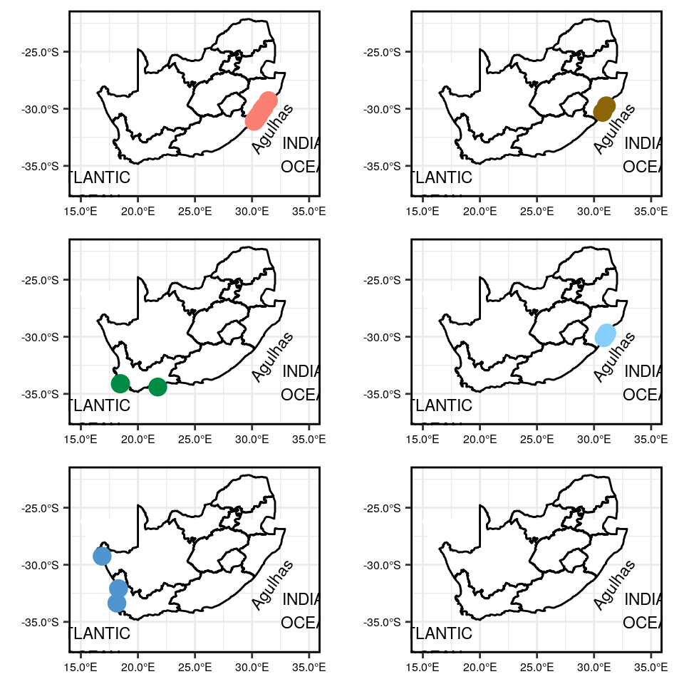

Figure 1: Maps showing closely related sites based on temperature variation at different regions along the coastline.

Calculating the distance between sites

Calculating the distance between each of the sites along the coastline. The deg2rad function transforms degrees to radians: Transforms between angles in degrees and radians.

options(scipen=999) # Forces R to not use exponential notation
sa_coast_prep <- sa_coast %>% 
  mutate(site = 1:nrow(.),
         X = deg2rad(X),
         Y = deg2rad(Y)) %>% 
  select(site, X, Y)

sa_coast_dist <- as.data.frame(round(PairsDists(sa_coast_prep), 2)) %>% 
  mutate(lon = sa_coast$X,
         lat = sa_coast$Y) %>% 
  dplyr::rename(dist = V1) %>%
  select(lon, lat, dist) %>% 
  mutate(cum_dist = cumsum(dist)) %>% 
  mutate(dist = lag(dist),
         cum_dist = lag(cum_dist))

Matching sites

Creating a function to match the sites with in a cluster: This function allows me to match sites within the same cluster based on the date that temperature was collected. This allows me to compare whether or not a temperature variation exist between sites within the same cluster and to examine various reasons for this variation. Here we consider distance between sites.

## testing...
# df <- SACTN_daily_clusters
# clust <- 1
##
clust_match <- function(df, clust) {
  SACTN_clust_x_match <- data.frame()
  df2 <- df %>%
    filter(cluster == clust) %>%
    select(-length) %>%
    droplevels()
  for (i in 1:length(levels(df2$index))) {  
    # for (i in 1:10) {
    SACTN_df_1 <- filter(df2, index == levels(index)[i])
    
    # Find the cumulative distance of site 1 along the coast
    site_dist_1 <- site_list_clusters %>% 
      filter(index == as.character(SACTN_df_1$index)[1])
    site_dist_1 <- knnx.index(data = as.matrix(sa_coast_dist[,1:2]),
                              query = as.matrix(site_dist_1[,5:6]), k = 1)
    site_dist_1 <- sa_coast_dist$cum_dist[site_dist_1]
    
    for (j in 1:length(levels(df2$index))) {
      # for(j in 1:10) {
      if (i == j) {
        next
      }
      if (j < i) {
        next
      }
      SACTN_df_2 <- filter(df2, index == levels(index)[j])
      
      # Find the cumulative distance of site 2 along the coast
      site_dist_2 <- site_list_clusters %>% 
        filter(index == as.character(SACTN_df_2$index)[1])
      site_dist_2 <- knnx.index(data = as.matrix(sa_coast_dist[,1:2]),
                                query = as.matrix(site_dist_2[,5:6]), k = 1)
      site_dist_2 <- sa_coast_dist$cum_dist[site_dist_2]
      
      # # The distance between the two sites
      site_dist_3 <- round(abs(site_dist_1-site_dist_2), 0)

      SACTN_df_3 <- left_join(SACTN_df_1, SACTN_df_2, by = "date") %>%
        na.trim() %>%
        select(date, index.x, temp.x, index.y, temp.y, -cluster.x, -cluster.y) %>%
        dplyr::rename(index_1 = index.x,
          temp_1 = temp.x,
          index_2 = index.y,
          temp_2 = temp.y) %>%
        mutate(index_pair = paste0(index_1, " - ", index_2, " - ", site_dist_3),
               index_dist = site_dist_3)
      SACTN_clust_x_match <- rbind(SACTN_clust_x_match, SACTN_df_3)
    }
  }
  return(SACTN_clust_x_match)
}


SACTN_clust_1_match <- clust_match(df = SACTN_daily_clusters_sub, clust = 1)
# SACTN_clust_2_match <- clust_match(df = SACTN_daily_clusters_sub, clust = 2)
# SACTN_clust_3_match <- clust_match(df = SACTN_daily_clusters_sub, clust = 3)
# SACTN_clust_4_match <- clust_match(df = SACTN_daily_clusters_sub, clust = 4)
# SACTN_clust_5_match <- clust_match(df = SACTN_daily_clusters_sub, clust = 5)
# SACTN_clust_6_match <- clust_match(df = SACTN_daily_clusters_sub, clust = 6)

Creating a function which allows me to calculated the monthly mean temperature and standard deviation for each year and sites. Consequently we have a data frame with 7 columns and each of the rows representing each month for each of the years. By calculating the mean and SD for each site i am able identify trends in their temperatures and to compare these trends across sites within the same cluster. Mean and SD gives a broad look of the overall temperature for each of the sites. With each group of months representing the season.

# Calculate all of the matche-ups in cluster 1

clust_matched <- function(df) {
  SACTN_clust_x_matched <- df %>%
  mutate(temp_matched = temp_1-temp_2,
         month = month(date, abbr = T, label = T),
         year = year(date)) %>%
  select(-temp_1, -temp_2) %>%
  group_by(index_pair, index_dist, month, year) %>%
  summarise(temp_mean_month_year = mean(temp_matched, na.rm = T),
            temp_sd_month_year = sd(temp_matched, na.rm = T)) %>% 
    mutate(season = ifelse(month %in% c("Jan", "Feb", "Mar"), "Summer",        
                           ifelse(month %in% c("Apr", "May", "Jun"), "Autumn",
                                ifelse(month %in% c("Jul", "Aug", "Sep"), "Winter",
                                       ifelse(month %in% c("Oct", "Nov", "Dec"), "Spring","Error")))))
  return(SACTN_clust_x_matched)
}

SACTN_clust_1_matched <- clust_matched(df = SACTN_clust_1_match)
# SACTN_clust_2_matched <- clust_matched(df = SACTN_clust_2_match)
# SACTN_clust_3_matched <- clust_matched(df = SACTN_clust_3_match)
# SACTN_clust_4_matched <- clust_matched(df = SACTN_clust_4_match)
# SACTN_clust_5_matched <- clust_matched(df = SACTN_clust_5_match)
# SACTN_clust_6_matched <- clust_matched(df = SACTN_clust_6_match)

Amieroh Abrahams

Scientist with a passion for data, statistics; the ocean and the oceangraphic processes associated with it.